Stabilizing the Q-Gradient Field for Policy Smoothness in Actor-Critic Methods

Jeong Woon Lee*, Kyoleen Kwak*, Daeho Kim*, Hyoseok Hwang
{everyman123, 2007kkl, daeho, hyoseok}@khu.ac.kr
* Equal contribution   Corresponding author
Kyung Hee University AIRLAB
ICML 2026 (Spotlight)

Abstract

Policies learned via continuous actor-critic methods often exhibit erratic, high-frequency oscillations, making them unsuitable for physical deployment. Current approaches attempt to enforce smoothness by directly regularizing the policy's output. We argue that this approach treats the symptom rather than the cause. In this work, we theoretically establish that policy non-smoothness is fundamentally governed by the differential geometry of the critic. By applying implicit differentiation to the actor-critic objective, we prove that the sensitivity of the optimal policy is bounded by the ratio of the Q-function's mixed-partial derivative (noise sensitivity) to its action-space curvature (signal distinctness). To empirically validate this theoretical insight, we introduce Policy-Aware Value-field Equalization (PAVE), a critic-centric regularization framework that treats the critic as a scalar field and stabilizes its induced action-gradient field. PAVE rectifies the learning signal by minimizing the Q-gradient volatility while preserving local curvature. Experimental results demonstrate that PAVE achieves smoothness comparable to policy-side smoothness regularization methods, while maintaining competitive task performance, without modifying the actor.

Method

Theoretical Analysis: The Geometry of Policy Sensitivity

To remediate the fundamental origin of action instability in actor-critic methods, we analyze how the differential geometry of the value function dictates the behavior of the induced policy. We derive the sensitivity of the greedy policy $a^{*}(s) = \arg\max_{a} Q(s, a)$ with respect to state perturbations and show, via the Implicit Function Theorem (IFT), that policy smoothness is governed by specific Hessian terms of the critic.

Implicit Policy Definition and Sensitivity Derivation

In the actor-critic paradigm, the actor $\pi_\phi(s)$ is optimized to approximate the maximizer of the Q-function. Even when the actor is a neural network, its update direction is fundamentally driven by $\nabla_a Q(s,\pi_\phi(s))$. The geometric regularity of the explicit maximizer $a^{*}(s) = \arg\max_{a} Q(s, a)$ therefore imposes a fundamental limit on the learned policy: $\pi_\phi$ cannot be smoother than $a^{*}$ without deviating from the optimal action.

Lemma 1 (Implicit Policy Jacobian).
Let $Q : \mathcal{S} \times \mathcal{A} \to \mathbb{R}$ be twice continuously differentiable. Assume that for a given state $s$, $a^{*}(s)$ is a strict local maximum and an interior point of $\mathcal{A}$, so that the action Hessian $\nabla^{2}_{aa} Q(s, a^{*}(s))$ is negative definite. Then the policy Jacobian $J_{\pi}(s) = \nabla_s a^{*}(s)$ is given analytically by $$ J_{\pi}(s) \;=\; -\bigl[\nabla^{2}_{aa} Q(s, a^{*}(s))\bigr]^{-1}\, \nabla^{2}_{sa} Q(s, a^{*}(s)). $$
Proof.
Since $a^{*}(s)$ is an interior extremum, it satisfies the first-order optimality condition $\nabla_a Q(s, a^{*}(s)) = 0$. Treating this as a vector-valued mapping $G(s, a(s)) = 0$, the total derivative with respect to $s$ gives, by the chain rule, $$ \nabla^{2}_{sa} Q(s, a^{*}(s)) \;+\; \nabla^{2}_{aa} Q(s, a^{*}(s))\, \nabla_s a^{*}(s) \;=\; 0. $$ By the strict-concavity assumption, $\nabla^{2}_{aa} Q(s, a^{*}(s))$ is invertible. Pre-multiplying by its inverse yields the stated formula. $\blacksquare$
Remark.
Lemma 1 requires $a^{*}(s)$ to be an interior strict local maximum. When optimal actions lie on the boundary of $\mathcal{A}$ or are not unique, the implicit function theorem does not apply and $J_\pi(s)$ may not be well-defined. In practice, continuous-control environments with $\tanh$-bounded actions rarely saturate the boundary, and our empirical results confirm that the regularization motivated by this analysis remains effective even when the assumption is not universally satisfied.

Geometrically, policy sensitivity is the product of an inverse curvature term and a mixed-partial coupling term: $\nabla^{2}_{sa} Q$ acts as a forcing term that dictates how the ascent direction shifts under state perturbations, while $[\nabla^{2}_{aa} Q]^{-1}$ acts as an amplification factor determined by the flatness of the landscape. If the Q-surface is flat (low curvature), the inverse Hessian explodes, rendering the policy hypersensitive to even negligible gradient rotations.

Spectral Bounds on Lipschitz Continuity
Proposition 2 (Lipschitz Continuity Bound).
Let $\|\cdot\|_2$ denote the spectral norm. Suppose $\|\nabla^{2}_{sa} Q(s, a^{*}(s))\|_2 \le M$ and the action Hessian satisfies the strict concavity condition $\lambda_{\max}(\nabla^{2}_{aa} Q(s, a^{*}(s))) \le -\mu < 0$. Then the induced greedy policy is Lipschitz continuous with constant $L$ satisfying $$ \|a^{*}(s) - a^{*}(s')\|_2 \;\le\; L\, \|s - s'\|_2, \qquad L \;\le\; \frac{M}{\mu}. $$
Proof.
Apply the spectral norm to the policy Jacobian from Lemma 1 and use sub-multiplicativity: $$ \|J_\pi(s)\|_2 \;\le\; \bigl\|[\nabla^{2}_{aa} Q]^{-1}\bigr\|_2 \cdot \|\nabla^{2}_{sa} Q\|_2 . $$ (i) Curvature bound. The assumption $\lambda_{\max}(\nabla^{2}_{aa} Q) \le -\mu$ places the spectrum of the Hessian inside $(-\infty, -\mu]$. The eigenvalues of the inverse Hessian are therefore bounded in magnitude by $1/\mu$, giving $\bigl\|[\nabla^{2}_{aa} Q]^{-1}\bigr\|_2 \le 1/\mu$.
(ii) Mixed-partial bound. By hypothesis, $\|\nabla^{2}_{sa} Q\|_2 \le M$.
Substituting and taking the supremum over $s$, $L \triangleq \sup_{s} \|J_\pi(s)\|_2 \le M/\mu$. The Mean Value Inequality for vector-valued differentiable functions then gives $\|a^{*}(s) - a^{*}(s')\|_2 \le L\,\|s - s'\|_2 \le (M/\mu)\,\|s - s'\|_2$. $\blacksquare$
Remark.
The condition $\lambda_{\max}(\nabla^{2}_{aa} Q(s, a^{*}(s))) \le -\mu < 0$ may not hold everywhere for neural-network critics. In our experiments, unconstrained critics satisfy this condition in only 14–47% of visited states. The bound $L \le M/\mu$ therefore serves as a regularization motivation rather than a universal guarantee. PAVE's $\mathcal{L}_{\mathrm{Curv}}$ improves satisfaction to 64–100% across environments.
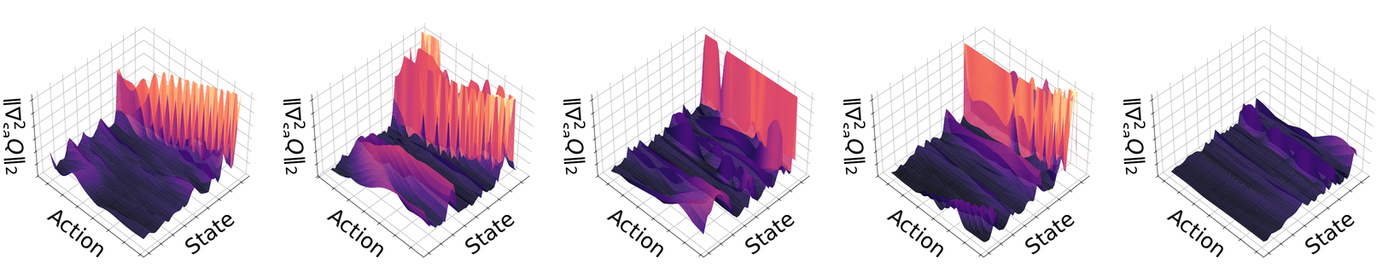
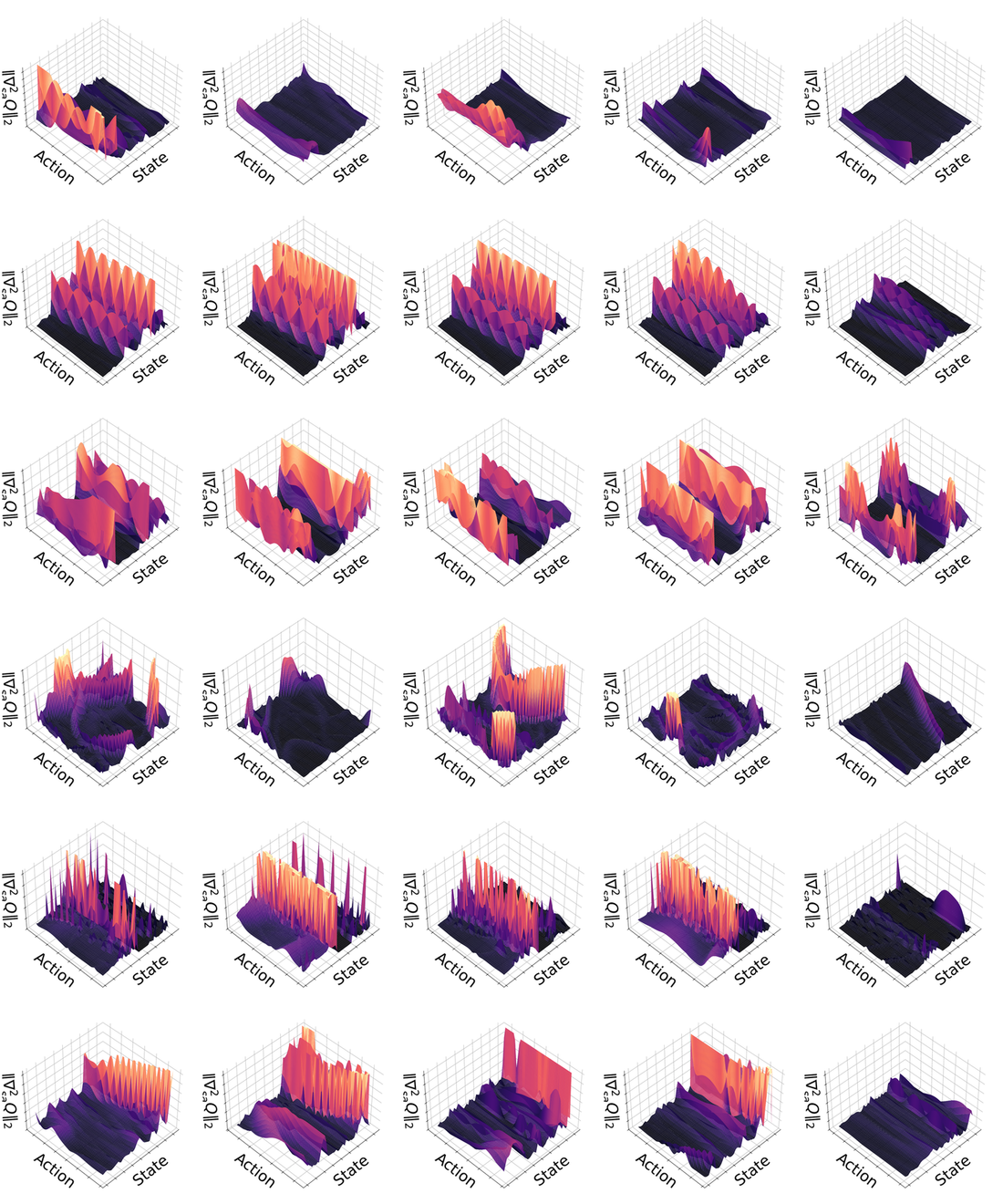
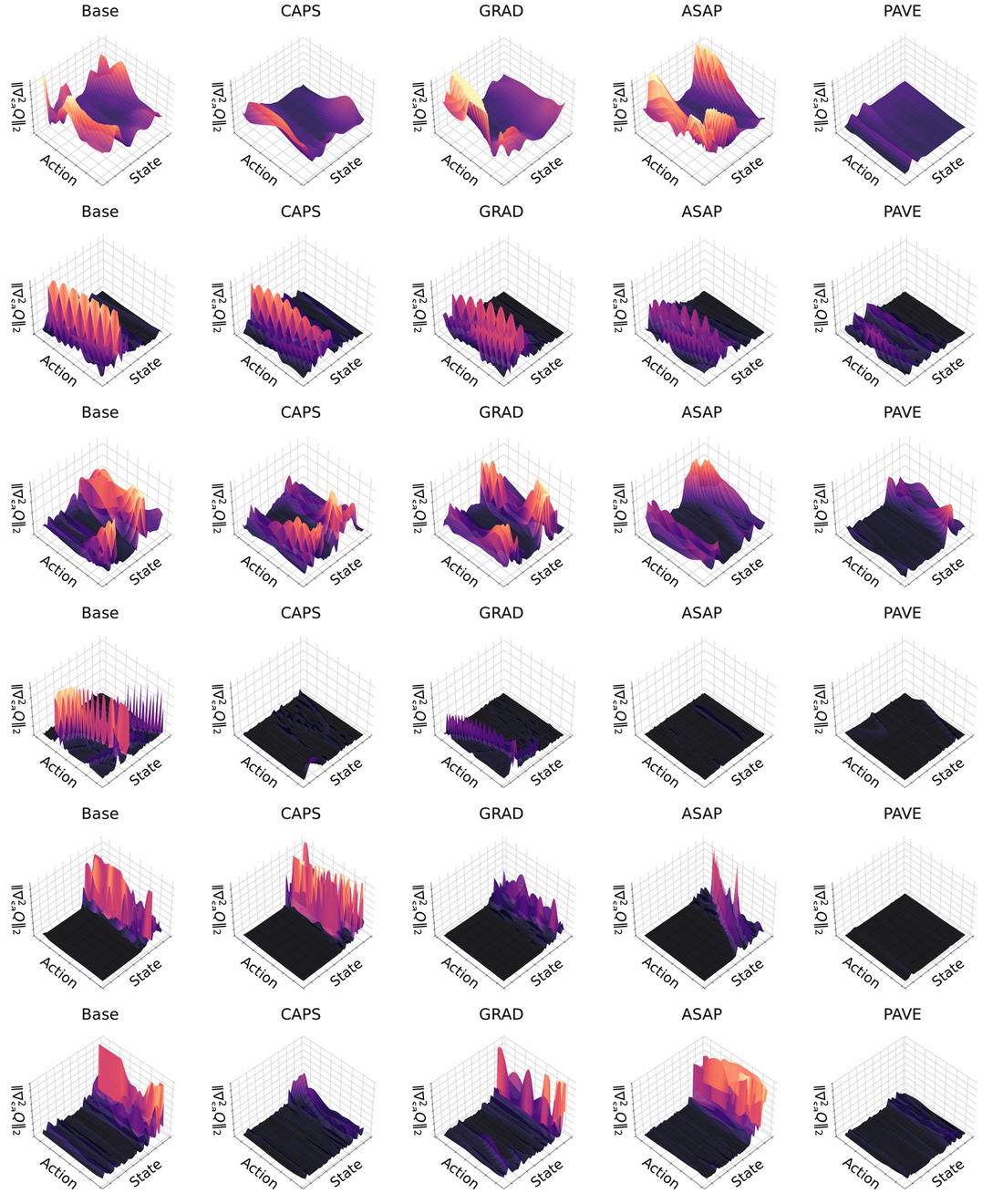
Theoretical implication. The bound $L \le M/\mu$ shows that simply minimizing the gradient variance (reducing $M$) is insufficient if the curvature $\mu$ also vanishes. Conventional regularizers tend to flatten the Q-landscape, driving $\mu \to 0$, which can theoretically explode the sensitivity term $\|[\nabla^{2}_{aa} Q]^{-1}\|$. PAVE is explicitly formulated to minimize $M$ while ensuring that $\mu$ stays strictly bounded away from zero.

PAVE: Policy-Aware Value-field Equalization

PAVE directly enforces the geometric stability conditions derived above. Instead of constraining the actor, PAVE regularizes the critic to minimize the Lipschitz bound $L \le M/\mu$ and to enforce trajectory consistency. This is achieved by three synergistic objectives: (1) suppressing noise sensitivity ($M$) via Mixed-Partial Regularization, (2) aligning temporal vector fields via Vector Field Consistency, and (3) preserving curvature ($\mu$) via Curvature Preservation to prevent geometric collapse. The losses below are finite-difference proxies that incentivize the desired geometric properties rather than guaranteeing them.

Mixed-Partial Regularization (MPR)

To minimize the numerator $M$ in the Lipschitz bound, we suppress the magnitude of $\nabla^{2}_{sa} Q$. Direct construction of the mixed Hessian costs $\mathcal{O}(d^{2})$, which is prohibitive online. We instead use a finite-difference proxy grounded in a Taylor expansion. Considering a small state perturbation $\epsilon$, $$ \nabla_a Q(s+\epsilon, a) \;=\; \nabla_a Q(s, a) + \nabla^{2}_{sa} Q(s,a)\,\epsilon + \mathcal{O}(\|\epsilon\|^{2}), $$ so $\|\nabla_a Q(s+\epsilon, a) - \nabla_a Q(s, a)\|$ is an efficient proxy for the Hessian-vector product $\|\nabla^{2}_{sa} Q\,\epsilon\|$. This motivates

$$ \mathcal{L}_{\mathrm{MPR}}(\theta) \;=\; \mathbb{E}_{\substack{(s,a)\sim\mathcal{D}\\ \epsilon \sim \mathcal{N}(0,\sigma^{2}I)}} \Bigl[\; \bigl\| \nabla_a Q(s+\epsilon, a) - \nabla_a Q(s, a) \bigr\|_2^{2} \;\Bigr]. $$

Formal justification. Substituting the linear approximation and integrating over the isotropic Gaussian noise $\epsilon$, $$ \mathcal{L}_{\mathrm{MPR}} \;\approx\; \mathbb{E}_\epsilon\!\left[\,\epsilon^{\top} (\nabla^{2}_{sa} Q)^{\top} (\nabla^{2}_{sa} Q)\, \epsilon\,\right] \;=\; \sigma^{2}\,\|\nabla^{2}_{sa} Q\|_F^{2}. $$ Since the spectral norm is upper-bounded by the Frobenius norm ($\|A\|_2 \le \|A\|_F$), minimizing $\mathcal{L}_{\mathrm{MPR}}$ encourages a smaller upper bound on $M$.

Vector Field Consistency (VFC)

MPR enforces spatial smoothness via isotropic perturbations, but stable robotic control also requires temporal coherence along trajectories. Interpreting $\nabla_a Q(s, a)$ as the score function of an implicit Boltzmann policy $p(a\mid s) \propto \exp(Q(s,a))$, we frame temporal stability as minimizing the distributional shift of the policy across consecutive states — a Fisher-divergence-style objective:

$$ \mathcal{L}_{\mathrm{VFC}}(\theta) \;=\; \mathbb{E}_{(s_t, a_t, s_{t+1}) \sim \mathcal{D}} \Bigl[\; \bigl\| \nabla_a Q(s_t, a_t) - \nabla_a Q(s_{t+1}, a_t) \bigr\|_2^{2} \;\Bigr]. $$

Formal justification. Using the first-order expansion $s_{t+1} \approx s_t + \Delta s_t$, $$ \bigl\|\nabla_a Q(s_{t+1}, a_t) - \nabla_a Q(s_t, a_t)\bigr\|_2^{2} \;\approx\; \bigl\|\nabla^{2}_{sa} Q(s_t, a_t)\, \Delta s_t\bigr\|_2^{2}. $$ Whereas MPR reduces $M$ globally, VFC encourages a smaller $M$ specifically along the state transitions imposed by the environment dynamics ($\nabla^{2}_{sa} Q\,\Delta s_t$). This mitigates the "chattering" effect caused by conflicting gradients at adjacent timesteps.

Curvature Preservation (Curv)

Minimizing $\mathcal{L}_{\mathrm{MPR}}$ in isolation introduces a pathological risk: the network may collapse $Q$ to a trivial flat plane (i.e.\ $\nabla_a Q \approx 0$ everywhere) to satisfy the smoothness penalty. By Proposition 2, if $Q$ becomes flat, $\|[\nabla^{2}_{aa} Q]^{-1}\|$ diverges, paradoxically amplifying policy sensitivity. To preclude this "over-smoothing" collapse, we enforce a curvature lower bound:

$$ \mathcal{L}_{\mathrm{Curv}}(\theta) \;=\; \mathbb{E}_{\substack{(s,a) \sim \mathcal{D}\\ v \sim p(v)}} \Bigl[\; \max\!\bigl(0,\; v^{\top} \nabla^{2}_{aa} Q(s, a)\, v + \delta \bigr) \;\Bigr], $$

where $\delta > 0$ is the minimum required sharpness. Computational efficiency is preserved by Hutchinson's trace estimator with random Rademacher vectors $v$. To enable a valid Hessian computation we use SiLU activations in the critic to ensure $C^{2}$ continuity.

Formal justification. This regularizer explicitly targets the denominator $\mu$ in the Lipschitz bound $L \le M/\mu$. By penalizing projected curvature values $v^{\top} \nabla^{2}_{aa} Q\, v$ that exceed $-\delta$, this objective incentivizes concavity via Hutchinson's trace estimator, which controls the trace rather than individual eigenvalues. This encourages the maximum eigenvalue to remain negative, helping to keep the inverse Hessian norm bounded and reducing sensitivity.

Total Objective

The composite objective for the critic parameter $\theta$ is a weighted sum of the standard temporal-difference regression loss and the three geometric regularizers:

$$ \mathcal{L}(\theta) \;=\; \mathcal{L}_{\mathrm{TD}}(\theta) \;+\; \lambda_{1}\, \mathcal{L}_{\mathrm{MPR}}(\theta) \;+\; \lambda_{2}\, \mathcal{L}_{\mathrm{VFC}}(\theta) \;+\; \lambda_{3}\, \mathcal{L}_{\mathrm{Curv}}(\theta). $$

Crucially, these geometric regularizers are applied solely as auxiliary losses to the critic. The actor update mechanism remains unchanged, using standard policy gradients while benefiting from the paved, well-conditioned Q-gradient landscape.

Quantitative Results

We evaluate PAVE on six Gymnasium / MuJoCo continuous-control environments (LunarLander, Pendulum, Reacher, Ant, Hopper, Walker2d) under both TD3 and SAC. All methods, including baselines, are re-trained with SiLU activations ("SiLU-unified") to remove confounders from the activation choice. We report cumulative return ($re$, higher is better) and the FFT-based smoothness score ($sm$, lower is better) following Mysore et al. (2021) and Christmann et al. (2024). Standard deviations are over five independent runs. Bold indicates the best and underline the second-best per environment.

Table 1. TD3 (SiLU-unified)
Method LunarLander Pendulum Reacher Ant Hopper Walker
$re\uparrow$$sm\downarrow$ $re\uparrow$$sm\downarrow$ $re\uparrow$$sm\downarrow$ $re\uparrow$$sm\downarrow$ $re\uparrow$$sm\downarrow$ $re\uparrow$$sm\downarrow$
Base 227.8
(74.1)
1.809
(1.311)
−168.7
(77.9)
1.590
(0.571)
−3.55
(1.32)
0.053
(0.014)
4299
(1499)
2.039
(0.400)
3056
(888)
2.715
(0.483)
4834
(423)
1.990
(0.208)
CAPS 249.0
(40.3)
0.702
(0.291)
−175.2
(79.3)
0.464
(0.165)
−3.58
(1.35)
0.047
(0.011)
4624
(1190)
2.135
(0.256)
3609
(33)
1.919
(0.373)
4913
(1383)
1.600
(0.306)
GRAD 245.1
(73.4)
0.669
(0.184)
−167.6
(75.6)
0.689
(0.139)
−3.55
(1.36)
0.041
(0.012)
5538
(845)
1.796
(0.187)
3317
(648)
1.642
(0.405)
4788
(783)
1.366
(0.194)
ASAP 168.4
(147.0)
2.055
(1.300)
−170.2
(80.7)
1.970
(0.768)
−3.56
(1.35)
0.051
(0.014)
4765
(1554)
2.065
(0.413)
3229
(553)
1.991
(0.259)
4740
(799)
1.616
(0.284)
PAVE 264.5
(24.9)
0.541
(0.290)
−167.6
(77.5)
0.351
(0.118)
−4.02
(1.34)
0.039
(0.013)
4649
(1443)
1.768
(0.315)
3305
(461)
0.950
(0.285)
5563
(451)
1.272
(0.172)

In the TD3 setting, the results validate the theoretical premise that stabilizing the Q-gradient field naturally induces policy smoothness without sacrificing performance. While baseline methods often exhibited a trade-off where improved smoothness came at the cost of reduced returns, PAVE consistently maintained or improved task performance. Most notably, on Walker, PAVE achieved both the highest cumulative return ($re = 5563$) and the best smoothness score ($sm = 1.272$). For deterministic policies, which are particularly prone to overfitting to sharp gradient irregularities, rectifying the critic's geometry proves to be a highly effective strategy.

Table 2. SAC (SiLU-unified)
Method LunarLander Pendulum Reacher Ant Hopper Walker
$re\uparrow$$sm\downarrow$ $re\uparrow$$sm\downarrow$ $re\uparrow$$sm\downarrow$ $re\uparrow$$sm\downarrow$ $re\uparrow$$sm\downarrow$ $re\uparrow$$sm\downarrow$
SAC Base 160.3
(135.3)
0.434
(0.187)
−163.1
(74.5)
0.548
(0.173)
−3.73
(1.37)
0.053
(0.016)
5276
(1029)
1.941
(0.289)
3481
(98)
0.773
(0.069)
4907
(283)
0.748
(0.063)
CAPS 270.9
(19.6)
0.271
(0.051)
−166.1
(76.9)
0.338
(0.118)
−3.69
(1.32)
0.048
(0.014)
5447
(884)
1.843
(0.241)
3442
(52)
0.660
(0.110)
4689
(178)
0.776
(0.071)
GRAD 256.6
(38.2)
0.252
(0.063)
−163.7
(74.5)
0.377
(0.111)
−3.74
(1.29)
0.046
(0.013)
5729
(604)
1.632
(0.103)
3315
(407)
0.581
(0.072)
4887
(211)
0.572
(0.052)
ASAP 268.6
(20.8)
0.183
(0.033)
−163.5
(74.7)
0.362
(0.109)
−3.66
(1.31)
0.048
(0.015)
5707
(852)
1.404
(0.088)
3077
(715)
0.404
(0.059)
4731
(209)
0.557
(0.069)
PAVE 265.8
(21.4)
0.142
(0.028)
−165.4
(75.5)
0.290
(0.130)
−3.71
(1.31)
0.052
(0.014)
5706
(774)
1.604
(0.146)
3489
(38)
0.556
(0.139)
4954
(250)
0.584
(0.020)

The SAC setting offers deeper insight into the characteristics of our method. In low-dimensional tasks such as Reacher, policy-side regularizers like GRAD and ASAP remain competitive in smoothness, suggesting that direct policy constraints are effective for simpler control manifolds; PAVE itself attains the best smoothness on LunarLander ($sm = 0.142$). However, the distinct advantage of PAVE emerges in high-dimensional environments with complex dynamics. On Walker, PAVE secures the highest cumulative return ($re = 4954$) while also achieving the strongest smoothness on LunarLander and Pendulum. On Ant, where GRAD achieves the highest return ($re = 5729$) at the cost of smoothness ($sm = 1.632$) and ASAP achieves the best smoothness ($sm = 1.404$) at a lower return, PAVE attains a competitive balance of both metrics ($re = 5706$, $sm = 1.604$). We attribute this to the fact that high-dimensional state–action spaces inherently exhibit more volatile curvature and frequent gradient spikes; in such chaotic landscapes, our critic-centric regularization effectively paves the optimization path, providing a stable learning signal that policy-side constraints alone fail to capture.

Takeaway. Across two off-policy backbones and six environments, PAVE wins or ties for the best smoothness in 8 / 12 settings while remaining competitive on cumulative return — without modifying the actor. This empirically confirms the theoretical prediction that policy non-smoothness can be addressed by reshaping the critic's differential geometry rather than by output-side regularization of the actor.

Empirical Validation of the Theory

The bound $L \le M / \mu$ in Proposition 2 makes a number of falsifiable predictions about how the critic's geometry should behave under regularization. This section tests them directly, using the additional experiments developed during the rebuttal process and now reported in the appendix of the paper.

(a) Does PAVE actually reduce $M$ and preserve $\mu$?

We compute the full mixed Hessian $\nabla^{2}_{sa} Q$ via autograd on trained critics and report $M_{\sup} = \sup\, \|\nabla^{2}_{sa} Q\|_{2}$ (largest singular value) as a measurement of $M$. We also report the negative-definiteness rate — the fraction of visited $(s, a)$ at which all eigenvalues of $\nabla^{2}_{aa} Q$ are strictly negative — as a measurement of whether the strict concavity assumption (and hence $\mu > 0$) holds in practice.

Method $M_{\sup} = \sup \|\nabla^{2}_{sa} Q\|_{2}\ \downarrow$
LunarPendReachAntHopWalk
Base99044716806788311923
CAPS121843124645210701624
GRAD127333818792024791990
ASAP1227393177964276271772
PAVE151210265962934643
Method Negative-definiteness rate of $\nabla^{2}_{aa} Q$\ $\uparrow$
LunarPendReachAntHopWalk
Base0.3520.4661.0000.1740.2590.141
PAVE0.8420.9950.9940.6590.8560.637

PAVE attains the lowest $M_{\sup}$ in 5 / 6 environments — a 2× to 9.5× reduction over Base — while simultaneously raising the strict-concavity satisfaction rate from 14–47 % under unregularized critics to 64–100 %. This is exactly the joint behaviour the bound $L \le M / \mu$ asks for: shrink the numerator, hold the denominator. Policy-side regularizers (CAPS, GRAD, ASAP) leave $M$ essentially untouched and in some cases (Hopper / ASAP) make it dramatically worse.

(b) Is the Q-gradient field actually geometrically unstable?

The theory motivates PAVE by claiming that the Q-gradient field $\nabla_a Q$ "rotates drastically with infinitesimal state perturbations". We test this directly by computing the cosine similarity between consecutive Q-gradients $\nabla_a Q(s_t, a_t)$ and $\nabla_a Q(s_{t+1}, a_{t+1})$ along rollouts. A negative cosine = a sign flip = the critic delivers contradictory update signals at adjacent states.

Env mean cosine $\uparrow$ flip rate ($\cos < 0$) $\downarrow$
BasePAVEBasePAVE
LunarLander0.5930.9010.1840.033
Pendulum0.4910.9540.2540.023
Reacher0.9500.9680.0160.010
Ant0.1530.1830.3550.333
Hopper0.5660.7550.1650.073
Walker0.6350.8350.0900.014

PAVE reduces the flip rate by 2–11× in 4 / 6 environments (Pendulum 25.4 % → 2.3 %, Walker 9.0 % → 1.4 %, LunarLander 18.4 % → 3.3 %, Hopper 16.5 % → 7.3 %). This is a direct empirical confirmation of the geometric-instability premise that the theory uses to motivate critic-side regularization.

(c) Critic-centric baselines: is it really $M$ and $\mu$?

The bound says reducing $M$ alone is not enough: if $\mu$ collapses, the inverse Hessian explodes and policy sensitivity actually grows. We test this by comparing PAVE against two existing critic-side regularizers that act on $M$-like quantities only:

  • SN-Critic — spectral normalization on the critic. Suppresses $M$ and $\mu$ indiscriminately.
  • GP-Critic — gradient penalty $\lambda \|\nabla_a Q\|^{2}$. Reduces $M$ but provides no mechanism for preserving $\mu$.
Method (Lunar / Walker, TD3+SiLU) $sm \downarrow$ $re \uparrow$ $M_{\sup} \downarrow$ Neg Def $\uparrow$
Base1.81 / 1.99228 / 4834990 / 19230.35 / 0.14
SN-Critic0.00 / 0.00−970 / 140.1 / —0.40 / 0.18
GP-Critic2.18 / 1.66202 / 5011882 / 10900.37 / 0.15
PAVE0.54 / 1.27264 / 5563151 / 6430.84 / 0.64

The result is exactly what the theory predicts. SN-Critic collapses both terms and trains a near-constant policy ($re = -970$ on Lunar). GP-Critic reduces $M$ moderately but leaves $\mu$ at the Base level, and its smoothness either worsens (Lunar) or improves only marginally (Walker). Only PAVE — which simultaneously suppresses $M$ via MPR/VFC and lower-bounds $\mu$ via Curv — attains both high return and low smoothness. The bound $L \le M / \mu$ is not a decoration: both terms must be controlled.

(d) $\mathcal{L}_{\mathrm{Curv}}$ is a prerequisite, not an option

A full $2^{3}$ factorial ablation of (MPR, VFC, Curv) on Walker isolates each term. The crucial row is MPR + VFC without Curv: removing the curvature term alone makes smoothness worse than the unregularized baseline.

Configuration Walker $re \uparrow$ Walker $sm \downarrow$
Base45891.828
MPR only50591.754
VFC only47881.823
MPR + VFC (no Curv)50102.095   (worse than Base!)
Curv only48961.650
MPR + Curv51771.718
VFC + Curv55371.918
MPR + VFC + Curv (Full PAVE)55021.483

This is a direct empirical confirmation of the theory: when only $M$ is suppressed, the network collapses curvature ($\mu \to 0$), the inverse Hessian $\bigl\| [\nabla^{2}_{aa} Q]^{-1} \bigr\|$ blows up, and policy sensitivity actually grows. Only the full PAVE objective — which guards the denominator with $L_{\mathrm{Curv}}$ — achieves the best smoothness and a competitive return.

(e) Does the actor still need its own smoothing?

Lemma 1 says the actor inherits the smoothness of the implicit greedy policy $a^{*}(s)$, which is determined entirely by the critic's geometry. If that argument is correct, adding an actor-side smoothness regularizer on top of PAVE should be essentially redundant. We test this by combining PAVE with CAPS, a representative actor-side smoothness regularizer, on LunarLander (TD3, SiLU):

Method $sm \downarrow$ $re \uparrow$
Base1.809227.8
CAPS (actor-side)0.702249.0
PAVE (critic-side)0.541264.5
CAPS + PAVE0.543264.0

PAVE alone already achieves the best smoothness and the best return; adding CAPS on top yields a virtually identical ($sm = 0.543$ vs $0.541$) outcome. Once the critic geometry is stabilized, the actor naturally tracks the implied smooth policy — no actor-side constraint is needed.

(f) Is the critic getting worse during training without PAVE?

Theory predicts that as TD-learning fits a more complex Q-surface, $\|\nabla^{2}_{sa} Q\|$ should grow over training unless something actively suppresses it. We checkpoint the critic at intermediate steps and recompute $M_{\sup}$ and the strict-concavity rate.

Env / step $M_{\sup} \downarrow$ Neg Def Rate $\uparrow$
BasePAVEBasePAVE
LunarLander — 100K2731010.2770.497
LunarLander — 300K6161290.2830.689
LunarLander — 500K11051880.3320.808
Walker — 200K6361670.0710.548
Walker — 600K12124170.1210.600
Walker — 1M13206590.1440.638

Base's $M_{\sup}$ grows by roughly over training on Lunar (273 → 1105) and stays large on Walker. PAVE keeps $M_{\sup}$ approximately constant (Lunar 101 → 188, <2×) and steadily improves the strict-concavity rate. The "unconstrained critic gets more volatile as it learns" is a real phenomenon, and PAVE counteracts it from early training onwards.

Putting it together. Across six independent angles — spectral $M$, concavity rate, cosine flips, critic-centric baselines, factorial ablation, actor-side combination, and training trajectory — the empirical picture is consistent with the bound $L \le M / \mu$ and with the claim that policy non-smoothness is a property of the critic's differential geometry. The same regularizer that provably targets $M$ and $\mu$ in theory also moves them in the right direction in practice, while baselines that target neither (policy-side) or only one (SN/GP-Critic) fail in the ways the theory predicts they should.

What "PAVing" the Q-Gradient Field Looks Like

The figures below visualise the spectral norm of the mixed Hessian, $\|\nabla^{2}_{sa} Q\|_2$, as a 3-D surface over a $50 \times 50$ sweep of (state dim, action dim). This is the empirical analogue of the theoretical bound $L \le M/\mu$: each peak marks an $(s, a)$ where a small state perturbation can rotate the action gradient sharply, directly upper-bounding how non-smooth any actor that climbs $\nabla_a Q$ can become. The dominant axis is selected once per environment from the Base critic and then re-used for every method, so the five panels in a row share the same axes. All panels share the same color scale (Z-axis clipped at the Base 99-th percentile) so heights are directly comparable.

Walker Q-gradient field — TD3, five methods.
Figure 1. Walker2d Q-gradient field under TD3, SiLU-unified. Left to right: Base, CAPS, GRAD, ASAP, PAVE. Baselines exhibit jagged landscapes with sharp spikes — this is the same $\|\nabla^{2}_{sa} Q\|$ that controls policy non-smoothness. PAVE flattens these spikes into a stable, paved manifold.

TD3 Q-gradient field grid across six environments.
Figure 2. Comprehensive Q-gradient field under TD3 (SiLU-unified). Rows top → bottom: LunarLander, Pendulum, Reacher, Ant, Hopper, Walker. Columns left → right: Base, CAPS, GRAD, ASAP, PAVE. PAVE has the lowest, smoothest surface in 5/6 environments, matching the quantitative reduction in $M_{\sup}$ reported in the paper.

SAC Q-gradient field grid across six environments.
Figure 3. Comprehensive Q-gradient field under SAC (SiLU-unified). Same protocol and ordering as Figure 2. The CAPS / GRAD / ASAP columns remain visually similar to Vanilla — policy-side regularizers smooth what the actor outputs but leave the critic's geometry essentially unchanged. Only PAVE acts on the geometry itself.

Conclusion

We identify the critic's irregular geometry as the root of policy instability. Using the Implicit Function Theorem, we prove that policy sensitivity is governed by the ratio of the Q-function's mixed-partial volatility to its action-space curvature, $L \le M/\mu$. To validate this insight we propose PAVE, which stabilizes this geometry via three lightweight, Hessian-free auxiliary critic losses. Empirical results confirm that paving the Q-gradient field induces smooth policies without actor-side constraints, substantiating the importance of a critic-centric perspective on continuous control.

BibTeX

@article{lee2026stabilizing,
  title={Stabilizing the Q-Gradient Field for Policy Smoothness in Actor-Critic},
  author={Lee, Jeong Woon and Kwak, Kyoleen and Kim, Daeho and Hwang, Hyoseok},
  journal={arXiv preprint arXiv:2601.22970},
  year={2026}
}